Plot OR

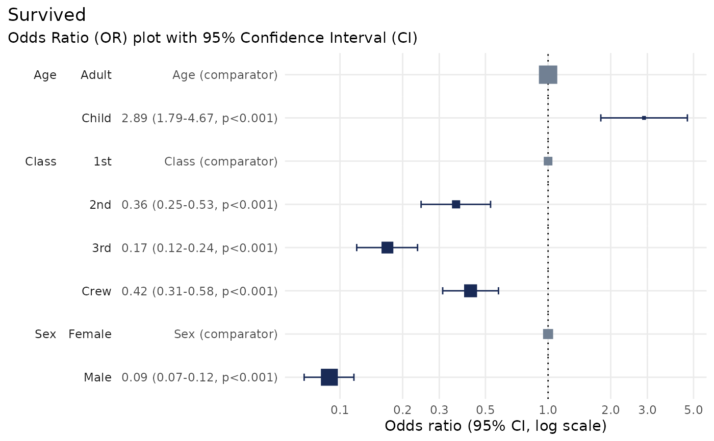
Produces an Odds Ratio plot to visualise the results of a logistic regression analysis.

Usage

plot_or(glm_model_results, conf_level = 0.95, confint_fast_estimate = FALSE)

Arguments

glm_model_results

Results from a binomial Generalised Linear Model (GLM), as produced by stats::glm().

conf_level

Numeric value between 0.001 and 0.999 (default = 0.95) specifying the confidence level for the confidence interval.

confint_fast_estimate

Boolean (default = FALSE) indicating whether to use a faster estimate of the confidence interval. Note: this assumes normally distributed data, which may not be suitable for your data.

Value

The function returns an object of class gg and ggplot, which can be customised and extended using various ggplot2 functions.

See also

• See vignette('using_plotor', package = 'plotor') for more details on usage.

• More details and examples can be found on the website: https://craig-parylo.github.io/plotor/index.html

Examples

# Load required libraries
library(plotor)
library(datasets)
library(dplyr)
#> 
#> Attaching package: ‘dplyr’
#> The following objects are masked from ‘package:stats’:
#> 
#>     filter, lag
#> The following objects are masked from ‘package:base’:
#> 
#>     intersect, setdiff, setequal, union
library(ggplot2)
library(stats)
library(forcats)
library(tidyr)

# Load the Titanic dataset
df <- datasets::Titanic |>
  as_tibble() |>
  # convert aggregated counts to individual observations
  filter(n > 0) |>
  uncount(weights = n) |>
  # convert character variables to factors
  mutate(across(where(is.character), as.factor))

# Perform logistic regression using `glm`
lr <- glm(
  data = df,
  family = 'binomial',
  formula = Survived ~ Class + Sex + Age
)

# Produce the Odds Ratio plot
plot_or(lr)