The goal of plotor is to generate Odds Ratio plots from logistic regression models.
Installation
You can install the development version of plotor from GitHub with:
# install.packages("devtools")
devtools::install_github("craig-parylo/plotor")
You can also install the latest released version from Cran with:
install.packages("plotor")
Example
In this example we will explore the likelihood of surviving the Titanic disaster based on passenger economic status (class), sex, and age group.
In addition to plotor
the packages we will use include dplyr
, tidyr
and forcats
for general data wrangling, the stats
package to conduct the logistic regression followed by broom
to tidy the output and convert the results to Odds Ratios and confidence intervals, then ggplot2
to visualise the plot.
library(plotor) # generates Odds Ratio plots
library(datasets) # source of example data
library(dplyr) # data wrangling
library(tidyr) # data wrangling - uncounting aggregated data
library(forcats) # data wrangling - handling factor variables
library(stats) # perform logistic regression using glm function
library(broom) # tidying glm model and producing OR and CI
library(ggplot2) # data visualisation
Start with getting the data from the datasets package.
df <- datasets::Titanic |>
as_tibble() |>
# convert counts to observations
filter(n > 0) |>
uncount(weights = n) |>
# convert categorical variables to factors.
# we specify an order for levels in Class and Survival, otherwise ordering
# in descending order of frequency
mutate(
Class = Class |>
fct(levels = c('1st', '2nd', '3rd', 'Crew')),
Sex = Sex |>
fct_infreq(),
Age = Age |>
fct_infreq(),
Survived = Survived |>
fct(levels = c('No', 'Yes'))
)
We now have a tibble of data containing four columns:
Survived
- our outcome variable describing whether the passenger survivedYes
or diedNo
,Class
- the passenger class, either1st
,2nd
,3rd
orCrew
,Sex
- the gender of the passenger, eitherMale
orFemale
,Age
- whether the passenger was anAdult
orChild
.
We next conduct a logistic regression of survival (as a binary factor: ‘yes’ and ‘no’) against the characteristics of passenger class, sex and age group. For this we use the Generalised Linear Model function (glm
) from the stats
package, specifying:
the family as ‘binomial’, and
the formula as survival being a function of
Class
,Sex
andAge
.
# conduct a logistic regression of survival against the other variables
lr <- glm(
data = df,
family = 'binomial',
formula = Survived ~ Class + Sex + Age
)
Finally, we can plot the Odds Ratio of survival using the plot_or
function.
# using plot_or
plot_or(glm_model_results = lr)
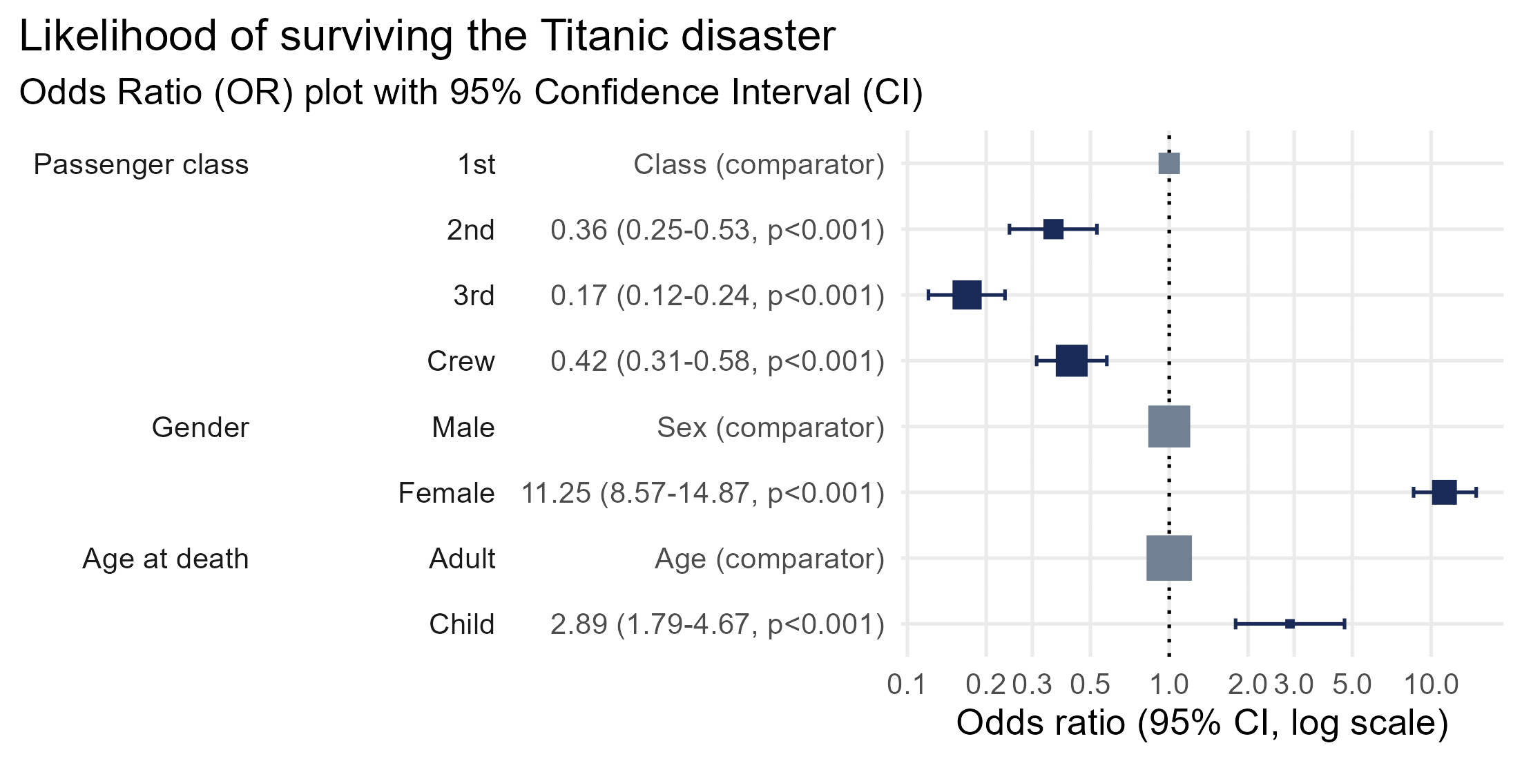
This plot makes it clear that:
Children were 2.89 times more likely to survive than Adults,
Passengers in
2nd
,3rd
class as well asCrew
were all less likely to survive than those in1st
class,Women were 11.25 times more likely to survive than men.