Creating publication-ready labels for your outputs

library(plotor)
set.seed(123)

Overview

By default, plot_or() and table_or() display variable names exactly as they appear in your model. Variable names like age_group_35_44 or smoking_status_yes are technical and not suitable for publication-ready outputs.

The solution is to attach human-readable labels to variables. When you do, plotor automatically uses these labels in plots and tables instead of the raw variable names. This approach is much cleaner than manually editing outputs after generation.

Example 1: Oesophageal Cancer Study

The dataset

This case-control study examined oesophageal cancer in Ile-et-Vilaine, France. It contains:

Variable	Description
`Group`	Case (cancer) or Control (disease-free)
`agegp`	Age group of participant
`alcgp`	Alcohol consumption (grams per day)
`tobgp`	Tobacco consumption (grams per day)

Preparing the data

# prepare the dataset for modelling
df <- 
  datasets::esoph |> 
  # convert aggregated data to tidy observational data
  tidyr::pivot_longer(
    cols = c(ncases, ncontrols),
    names_to = 'Group',
    values_to = 'people'
  ) |> 
  tidyr::uncount(weights = people) |> 
  # prepare the variables
  dplyr::mutate(
    # convert the intervention group to a factor
    Group = Group |> 
      dplyr::recode_values(
        "ncases" ~ "Case",
        "ncontrols" ~ "Control"
      ) |> 
        factor(levels = c("Control", "Case")),
    # remove ordering from these predictors
    agegp = agegp |> factor(ordered = FALSE),
    alcgp = alcgp |> factor(ordered = FALSE),
    tobgp = tobgp |> factor(ordered = FALSE)
  )

# preview the data
df |> dplyr::glimpse()
#> Rows: 975
#> Columns: 4
#> $ agegp <fct> 25-34, 25-34, 25-34, 25-34, 25-34, 25-34, 25-34, 25-34, 25-34, 2…
#> $ alcgp <fct> 0-39g/day, 0-39g/day, 0-39g/day, 0-39g/day, 0-39g/day, 0-39g/day…
#> $ tobgp <fct> 0-9g/day, 0-9g/day, 0-9g/day, 0-9g/day, 0-9g/day, 0-9g/day, 0-9g…
#> $ Group <fct> Control, Control, Control, Control, Control, Control, Control, C…

Without labels

m <- glm(
  data = df,
  family = "binomial",
  formula = Group ~ agegp + alcgp + tobgp
)

# plot the odds ratio with a customised title
plot_or(m)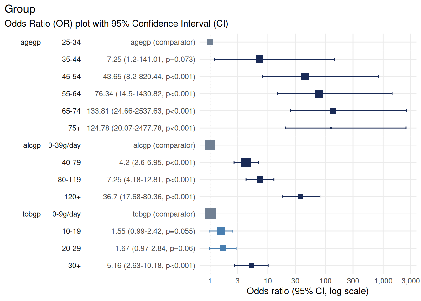

Notice how the plot uses technical variable names like alcgp and tobgp which are not immediately clear to readers.

Adding labels with `{labelled}`

To make your outputs more readable, attach descriptive labels to your variables before modelling.

First, ensure the package is installed.

install.packages("labelled")
library(labelled)

# create a list that matches variables with user-friendly labels
var_labels <- list(
  agegp = "Age group",
  alcgp = "Alcohol consumption",
  tobgp = "Tobacco consumption",
  Group = "Likelihood of developing oesophageal cancer"
)

# apply these variables to our data
labelled::var_label(df) <- var_labels

# preview the data with labels applied
labelled::look_for(df)
#>  pos variable label                                    col_type missing
#>  1   agegp    Age group                                fct      0      
#>                                                                        
#>                                                                        
#>                                                                        
#>                                                                        
#>                                                                        
#>  2   alcgp    Alcohol consumption                      fct      0      
#>                                                                        
#>                                                                        
#>                                                                        
#>  3   tobgp    Tobacco consumption                      fct      0      
#>                                                                        
#>                                                                        
#>                                                                        
#>  4   Group    Likelihood of developing oesophageal ca~ fct      0      
#>                                                                        
#>  values   
#>  25-34    
#>  35-44    
#>  45-54    
#>  55-64    
#>  65-74    
#>  75+      
#>  0-39g/day
#>  40-79    
#>  80-119   
#>  120+     
#>  0-9g/day 
#>  10-19    
#>  20-29    
#>  30+      
#>  Control  
#>  Case

Forest plots with labels

Now fit the model using the labelled data:

m <- glm(
  data = df,
  family = "binomial",
  formula = Group ~ agegp + alcgp + tobgp
)

# plot the odds ratio with a customised title
plot_or(m)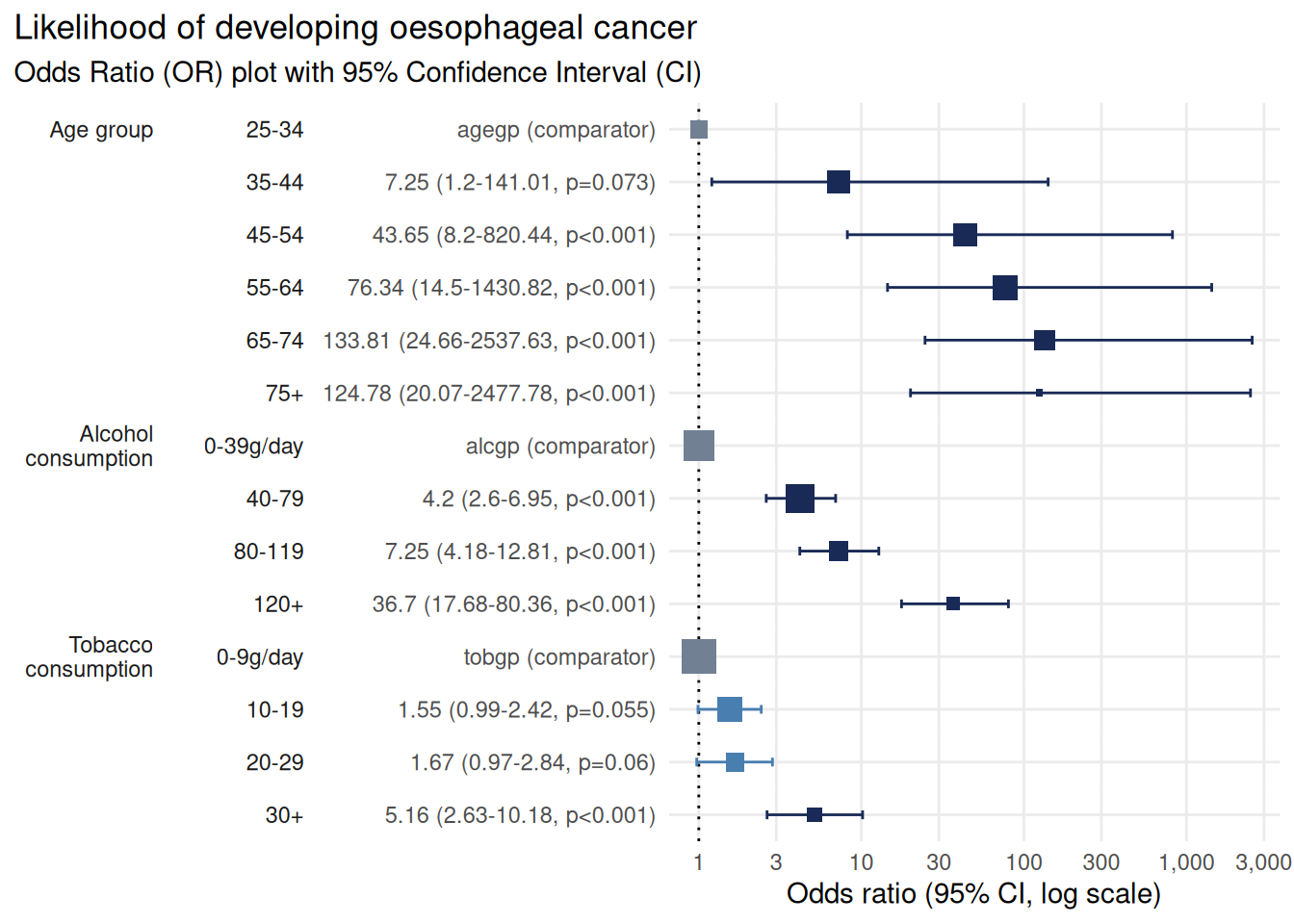

The plot is now much more reader-friendly:

The outcome label (“Likelihood of developing oesophageal cancer”) appears in the title
Predictor labels (“Age group”, “Alcohol consumption”, “Tobacco consumption”) replace technical variable names

Data tables with labels

table_or() also respects variable labels:

table_or(m, output = "gt", assumption_checks = FALSE)

	Characteristic¹					Odds Ratio (OR)²			95% Confidence Interval (CI)³			OR Plot
Likelihood of developing oesophageal cancer
Odds Ratio summary table with 95% Confidence Interval
	Level	N	n	Rate	Class	OR	SE	p	Lower	Upper	Significance	OR Plot
Age group	25-34	116	1	0.86%	factor	—	—	—	—	—	Comparator
	35-44	199	9	4.52%	factor	7.249	1.104	7.27 × 10⁻²	1.202	141.0	Significant
	45-54	213	46	21.6%	factor	43.65	1.068	4.06 × 10⁻⁴	8.204	820.4	Significant
	55-64	242	76	31.4%	factor	76.34	1.065	4.68 × 10⁻⁵	14.50	1,431	Significant
	65-74	161	55	34.16%	factor	133.8	1.076	5.38 × 10⁻⁶	24.66	2,538	Significant
	75+	44	13	29.55%	factor	124.8	1.121	1.67 × 10⁻⁵	20.07	2,478	Significant
Alcohol consumption	0-39g/day	415	29	6.99%	factor	—	—	—	—	—	Comparator
	40-79	355	75	21.13%	factor	4.198	0.2501	9.63 × 10⁻⁹	2.600	6.948	Significant
	80-119	138	51	36.96%	factor	7.248	0.2848	3.51 × 10⁻¹²	4.183	12.81	Significant
	120+	67	45	67.16%	factor	36.70	0.3850	8.19 × 10⁻²¹	17.68	80.36	Significant
Tobacco consumption	0-9g/day	525	78	14.86%	factor	—	—	—	—	—	Comparator
	10-19	236	58	24.58%	factor	1.550	0.2283	5.50 × 10⁻²	0.9885	2.423	Not significant
	20-29	132	33	25%	factor	1.670	0.2730	6.04 × 10⁻²	0.9714	2.839	Not significant
	30+	82	31	37.8%	factor	5.160	0.3441	1.85 × 10⁻⁶	2.631	10.18	Significant
¹ Characteristics are the explanatory variables in the logistic regression analysis. For categorical variables the first characteristic is designated as a reference against which the others are compared. For numeric variables the results indicate a change per single unit increase. Level - the name or the description of the explanatory variable. N - the number of observations examined. n - the number of observations resulting in the outcome of interest. Rate - the proportion of observations resulting in the outcome of interest (n / N). Class - description of the data type.
² Odds Ratios estimate the relative odds of an outcome with reference to the Characteristic. For categorical data the first level is the reference against which the odds of other levels are compared. Numerical characteristics indicate the change in OR for each additional increase of one unit in the variable. OR - The Odds Ratio point estimate - values below 1 indicate an inverse relationship whereas values above 1 indicate a positive relationship. Values shown to 4 significant figures. SE - Standard Error of the point estimate. Values shown to 4 significant figures. p - The p-value estimate based on the residual Chi-squared statistic.
³ Confidence Interval - the range of values likely to contain the OR in 95% of cases if this study were to be repeated multiple times. If the CI touches or crosses the value 1 then it is unlikely the Characteristic is significantly associated with the outcome. Lower & Upper - The range of values comprising the CI, shown to 4 significant figures. Significance - The statistical significance indicated by the CI, Significant where the CI does not touch or cross the value 1.

Example 2: Post-endoscopic pancreatitis study

The dataset

The indo_rct dataset contains details from 602 patients in a randomised controlled study examining indomethacin vs placebo for preventing post-endoscopic pancreatitis.

# prepare the dataset for modelling
df <- medicaldata::indo_rct |> 
  tibble::as_tibble() |> 
  # clean up factor levels
  dplyr::mutate(
    rx = forcats::fct_recode(
      .f = rx, 
      Placebo = "0_placebo", Indomethacin = "1_indomethacin"),
    pep = forcats::fct_recode(
      .f = pep,
      No = "0_no", Yes = "1_yes"
    ),
    amp = forcats::fct_recode(
      .f = amp,
      No = "0_no", Yes = "1_yes"
    )
  )

# fit the model without labels
m <- stats::glm(
  formula = outcome ~  rx + pep + amp,
  family = "binomial",
  data = df
)

plot_or(m, assumption_checks = FALSE)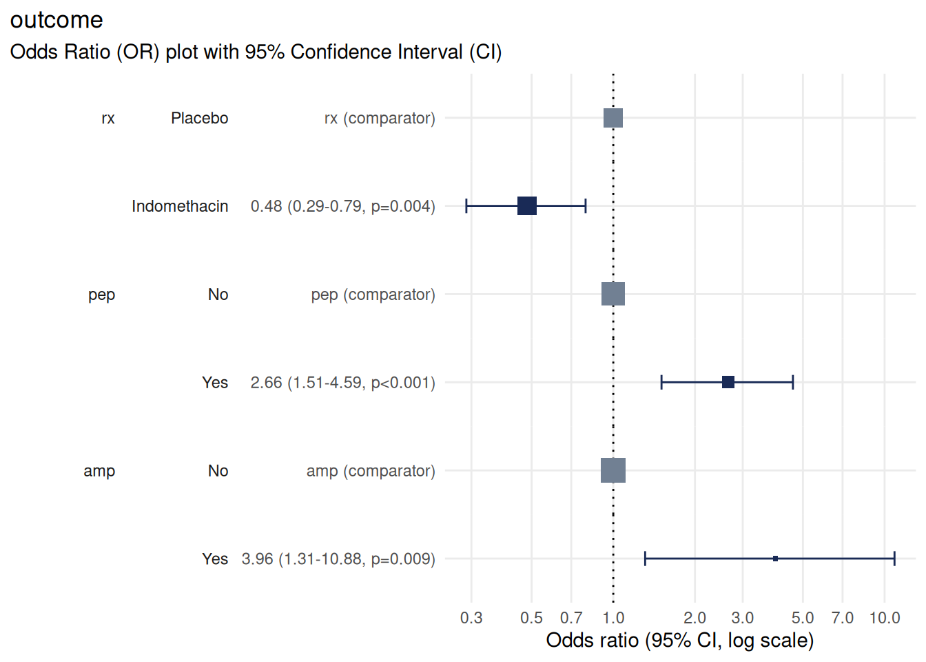

Using `{Hmisc}` for labels

An alternative to {labelled} is the {Hmisc} package, which is particularly useful if you’re already using other {Hmisc} functions like describe() for summary statistics.

Install it with:

install.packages("Hmisc")
library(Hmisc)

Attach labels using the label() function:

# label the variables
Hmisc::label(df$outcome) <- "Likelihood of post-ERCP pancreatitis"
Hmisc::label(df$rx) <- "Treatment arm"
Hmisc::label(df$pep) <- "Previous post-ERCP pancreatitis (PEP)"
Hmisc::label(df$amp) <- "Ampullectomy performed"

# fit the model with labelled data
m <- stats::glm(
  formula = outcome ~  rx + pep + amp,
  family = "binomial",
  data = df
)

# plot
plot_or(m, assumption_checks = FALSE)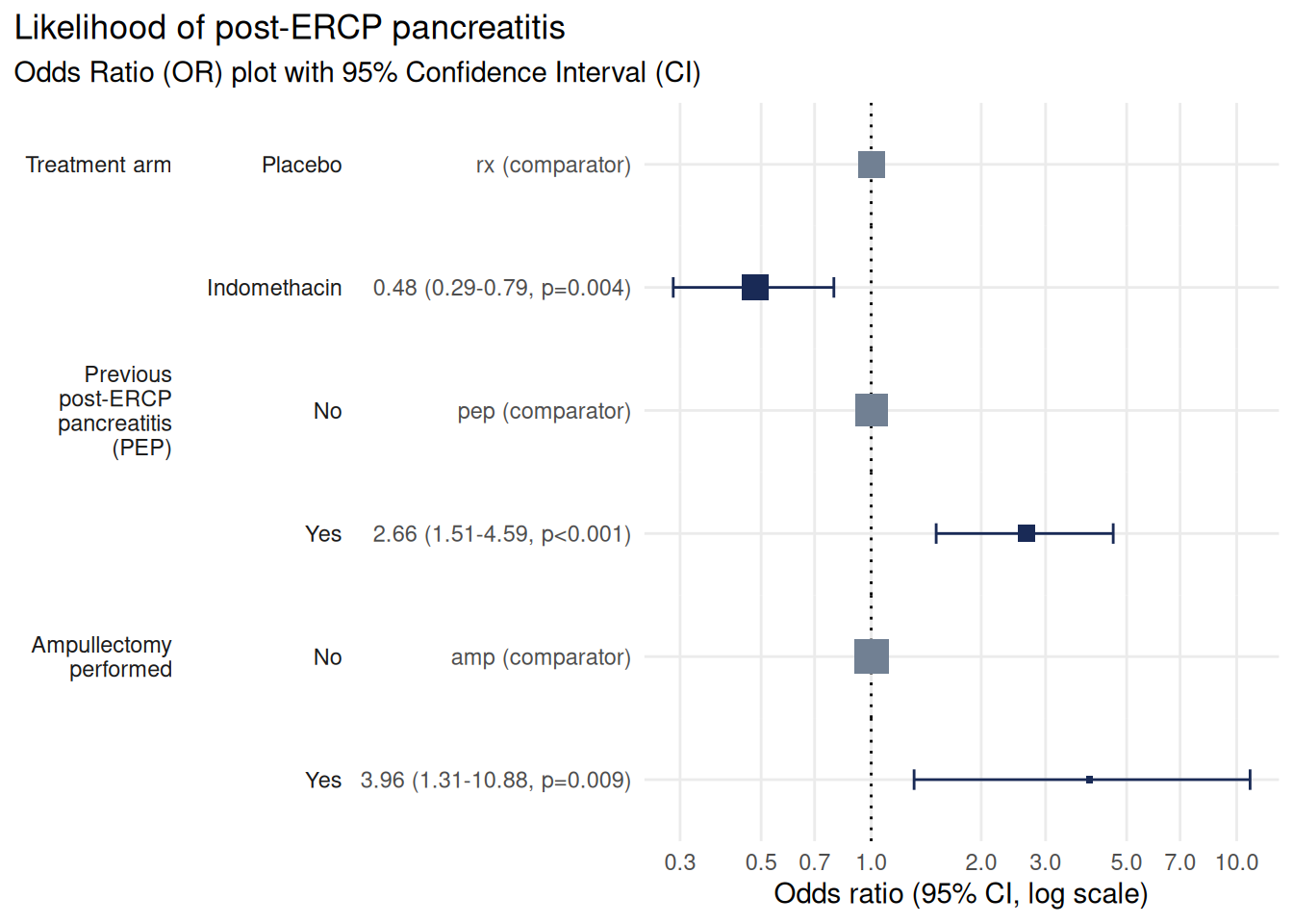

This plot now clearly shows that treatment with Indomethacin has a protective effect against pancreatitis, whereas a history of pancreatitis and ampullectomy are both associated with increased risk.

The same labels also appear in covariate tables:

table_or(m, output = "gt", assumption_checks = FALSE)

	Characteristic¹					Odds Ratio (OR)²			95% Confidence Interval (CI)³			OR Plot
Likelihood of post-ERCP pancreatitis
Odds Ratio summary table with 95% Confidence Interval
	Level	N	n	Rate	Class	OR	SE	p	Lower	Upper	Significance	OR Plot
Previous post-ERCP pancreatitis (PEP)	No	506	56	11.07%	labelled factor	—	—	—	—	—	Comparator
Previous post-ERCP pancreatitis (PEP)	Yes	96	23	23.96%	labelled factor	2.658	0.2834	5.61 × 10⁻⁴	1.506	4.594	Significant
Ampullectomy performed	No	584	73	12.5%	labelled factor	—	—	—	—	—	Comparator
Ampullectomy performed	Yes	18	6	33.33%	labelled factor	3.960	0.5306	9.49 × 10⁻³	1.310	10.88	Significant
Treatment arm	Placebo	307	52	16.94%	labelled factor	—	—	—	—	—	Comparator
Treatment arm	Indomethacin	295	27	9.15%	labelled factor	0.4816	0.2572	4.50 × 10⁻³	0.2874	0.7905	Significant
¹ Characteristics are the explanatory variables in the logistic regression analysis. For categorical variables the first characteristic is designated as a reference against which the others are compared. For numeric variables the results indicate a change per single unit increase. Level - the name or the description of the explanatory variable. N - the number of observations examined. n - the number of observations resulting in the outcome of interest. Rate - the proportion of observations resulting in the outcome of interest (n / N). Class - description of the data type.
² Odds Ratios estimate the relative odds of an outcome with reference to the Characteristic. For categorical data the first level is the reference against which the odds of other levels are compared. Numerical characteristics indicate the change in OR for each additional increase of one unit in the variable. OR - The Odds Ratio point estimate - values below 1 indicate an inverse relationship whereas values above 1 indicate a positive relationship. Values shown to 4 significant figures. SE - Standard Error of the point estimate. Values shown to 4 significant figures. p - The p-value estimate based on the residual Chi-squared statistic.
³ Confidence Interval - the range of values likely to contain the OR in 95% of cases if this study were to be repeated multiple times. If the CI touches or crosses the value 1 then it is unlikely the Characteristic is significantly associated with the outcome. Lower & Upper - The range of values comprising the CI, shown to 4 significant figures. Significance - The statistical significance indicated by the CI, Significant where the CI does not touch or cross the value 1.

Best practices for labelling

Be descriptive but concise

Keep labels clear and specific, but not verbose:

✓ Good	✗ Avoid
“Age Group (years)”	“The age of the participant in years”
“Systolic Blood Pressure (mmHg)”	“BP_sys”
“Smoking Status”	“smoking_status_yes”

Include units where relevant

Always specify units in parentheses:

var_labels <- list(
  wt = "Weight (kg)",
  ht = "Height (cm)",
  bp_sys = "Systolic Blood Pressure (mmHg)"
)

Use consistent formatting

Apply consistent capitalisation and punctuation across all labels:

# consistent approach to capitalisation
var_labels <- list(
  ag_gp = "Age Group",
  sm_status = "Smoking Status",
  ed_level = "Education Level"
)

Label factor levels clearly

Make factor level labels explicit and unambiguous:

df <-
  data.frame(
    education = sample(
      x = 1:3,
      size = 10,
      replace = TRUE
    ) |>
      factor(
        labels = c(
          "Primary school",
          "Secondary school",
          "University degree"
        )
      )
  )

Preserving labels in your workflow

R-native formats preserve labels

Labels are preserved when saving and reloading with .Rds or .RData:

# labels are preserved
saveRDS(df, "my_data.Rds")
df <- readRDS("my_data.Rds")

CSV files lose labels

Labels are lost when reading from CSV or other text formats. To preserve labels, use one of these approaches:

Use R-native formats like .Rds or .RData
Re-apply labels after reading CSV files
Store labels separately in a data dictionary and apply them in your analysis script

Overview

Example 1: Oesophageal Cancer Study

The dataset

Preparing the data

Without labels

Adding labels with {labelled}

Forest plots with labels

Data tables with labels

Example 2: Post-endoscopic pancreatitis study

The dataset

Using {Hmisc} for labels

Best practices for labelling

Be descriptive but concise

Include units where relevant

Use consistent formatting

Label factor levels clearly

Preserving labels in your workflow

R-native formats preserve labels

CSV files lose labels

See also

Adding labels with `{labelled}`

Using `{Hmisc}` for labels