Short summary: minimal reproducible workflow showing model checks, a publication-ready odds ratio table and a forest plot.
What this vignette covers
- Required input: a fitted glm object for binary outcome (family = binomial)
- Functions shown:
check_or(),table_or()andplot_or()
- Output types demonstrated: tibble, gt table, ggplot2 plot.
Minimal reproducible example
Create a small example dataset with clear factor levels and a binary outcome:
rows <- 400
df <- data.frame(
  # the first factor level is the reference,
  # results in odds of 'Disease' vs 'Healthy'
  outcome = rbinom(n = rows, size = 1, prob = 0.25) |>
    factor(labels = c("Healthy", "Disease")),
  age = rnorm(n = rows, mean = 50, sd = 12),
  sex = sample(x = 0:1, size = rows, replace = TRUE) |>
    factor(labels = c("Female", "Male")),
  smoke = sample(x = 0:2, size = rows, replace = TRUE) |>
    factor(labels = c("Never", "Former", "Current"))
)
Fit a logistic regression model
m <- glm(
  formula = outcome ~ age + sex + smoke,
  data = df,
  family = "binomial"
)
Run diagnostics
Using check_or()
check_or(m)
#>
#> ── Assumption checks ───────────────────────────────────────────────────────────
#>
#> ── Summary ──
#>
#> ✔ The outcome variable is binary
#> ✔ Predictor variables are not highly correlated with each other
#> ✔ The outcome is not separated by predictors
#> ✔ The sample size is large enough
#> ✔ Continuous variables either have a linear relationship with the log-odds of
#> the outcome or are absent
#> ✔ No observations unduly influence model estimates
#>
#> Your model was checked for logistic regression assumptions in the following
#> areas:
#>
#> Binary outcome:
#> The outcome variable was checked for containing precisely two levels.
#>
#> Multicollinearity:
#> The `vif()` function from the car package was used to check for highly
#> correlated predictor variables.
#>
#> Separation:
#> The `detectseparation()` function from the detectseparation package was used to
#> check for complete or quasi-complete separation in the data.
#>
#> Sample size:
#> A rule of thumb was applied, requiring at least 10 events per predictor
#> variable and at least 10 events per level of categorical variables to ensure
#> sufficient data for reliable estimates.
#>
#> Linearity:
#> A likelihood ratio test was conducted to assess improvements in model fit
#> compared to a model using Box-Tidwell power transformations on continuous
#> predictors. Any observed improvement likely indicates non-linear relationships
#> between the continuous predictors and the log-odds of the outcome.
#>
#> Influential observations:
#> A test to identify observations that could disproportionately influence model
#> statistics was applied. The test simultaneously examined three metrics: Cook's
#> distance (measuring overall observation impact), leverage (quantifying an
#> observation's distance from the data centre), and standardised residuals
#> (indicating how unusual an observation is relative to the model). To minimise
#> false positive, an observation was flagged only if it met at least two of these
#> diagnostic criteria.
#>
#> ✔ These tests found no issues with your model.
#>
Runs quick checks (binary outcome, multicollinearity, separation, small-sample / rare-event, linearity, influential points)
Behaviour: prints concise human-readable messages to the console
Issues raised here may indicate you should undertake further work to validate your model and understand the causes of these alerts before relying on any results from your model.
Create a publication-ready table
Using table_or()
# two output formats shown: gt (rendered) and tibble (for programmatic use)
table_or(m, output = "gt") # formatted HTML table| outcome | ||||||||||||
| Odds Ratio summary table with 95% Confidence Interval | ||||||||||||
Characteristic1
|
Odds Ratio (OR)2
|
95% Confidence Interval (CI)3
|
OR Plot | |||||||||
|---|---|---|---|---|---|---|---|---|---|---|---|---|
| Level | N | n | Rate | Class | OR | SE | p | Lower | Upper | Significance | ||
| age | age | 400 | 97 | 24.25% | numeric | 0.9897 | 0.009961 | 3.00 × 10⁻¹ | 0.9705 | 1.009 | Not significant | |
| sex | Female | 206 | 53 | 25.73% | factor | — | — | — | — | — | Comparator | |
| Male | 194 | 44 | 22.68% | factor | 0.8558 | 0.2350 | 5.07 × 10⁻¹ | 0.5385 | 1.355 | Not significant | ||
| smoke | Never | 137 | 34 | 24.82% | factor | — | — | — | — | — | Comparator | |
| Former | 135 | 34 | 25.19% | factor | 1.028 | 0.2808 | 9.21 × 10⁻¹ | 0.5923 | 1.786 | Not significant | ||
| Current | 128 | 29 | 22.66% | factor | 0.9018 | 0.2903 | 7.22 × 10⁻¹ | 0.5085 | 1.592 | Not significant | ||
|
1
Characteristics are the explanatory variables in the logistic regression analysis. For categorical variables the first characteristic is designated as a reference against which the others are compared. For numeric variables the results indicate a change per single unit increase.
Level - the name or the description of the explanatory variable. N - the number of observations examined. n - the number of observations resulting in the outcome of interest. Rate - the proportion of observations resulting in the outcome of interest (n / N). Class - description of the data type. |
||||||||||||
|
2
Odds Ratios estimate the relative odds of an outcome with reference to the Characteristic. For categorical data the first level is the reference against which the odds of other levels are compared. Numerical characteristics indicate the change in OR for each additional increase of one unit in the variable.
OR - The Odds Ratio point estimate - values below 1 indicate an inverse relationship whereas values above 1 indicate a positive relationship. Values shown to 4 significant figures. SE - Standard Error of the point estimate. Values shown to 4 significant figures. p - The p-value estimate based on the residual Chi-squared statistic. |
||||||||||||
|
3
Confidence Interval - the range of values likely to contain the OR in 95% of cases if this study were to be repeated multiple times. If the CI touches or crosses the value 1 then it is unlikely the Characteristic is significantly associated with the outcome.
Lower & Upper - The range of values comprising the CI, shown to 4 significant figures. Significance - The statistical significance indicated by the CI, Significant where the CI does not touch or cross the value 1. |
||||||||||||
table_or(m, output = "tibble") # programmatic output
#> # A tibble: 6 × 14
#>   label level    rows outcome outcome_rate class   estimate std.error statistic
#>   <fct> <fct>   <int>   <int>        <dbl> <chr>      <dbl>     <dbl>     <dbl>
#> 1 age   age       400      97        0.242 numeric    0.990   0.00996   -1.04
#> 2 sex   Female    206      53        0.257 factor    NA      NA         NA
#> 3 sex   Male      194      44        0.227 factor     0.856   0.235     -0.663
#> 4 smoke Never     137      34        0.248 factor    NA      NA         NA
#> 5 smoke Former    135      34        0.252 factor     1.03    0.281      0.0997
#> 6 smoke Current   128      29        0.227 factor     0.902   0.290     -0.356
#> # ℹ 5 more variables: p.value <dbl>, conf.low <dbl>, conf.high <dbl>,
#> #   significance <chr>, comparator <dbl>
Notes:
table_or() exponentiates coefficients to present odds ratios
Use the tibble output when you need to further transform or combine results programmatically
Forest plot of odds ratios
Display the relationships in a forest plot using plot_or()
plot_or(m)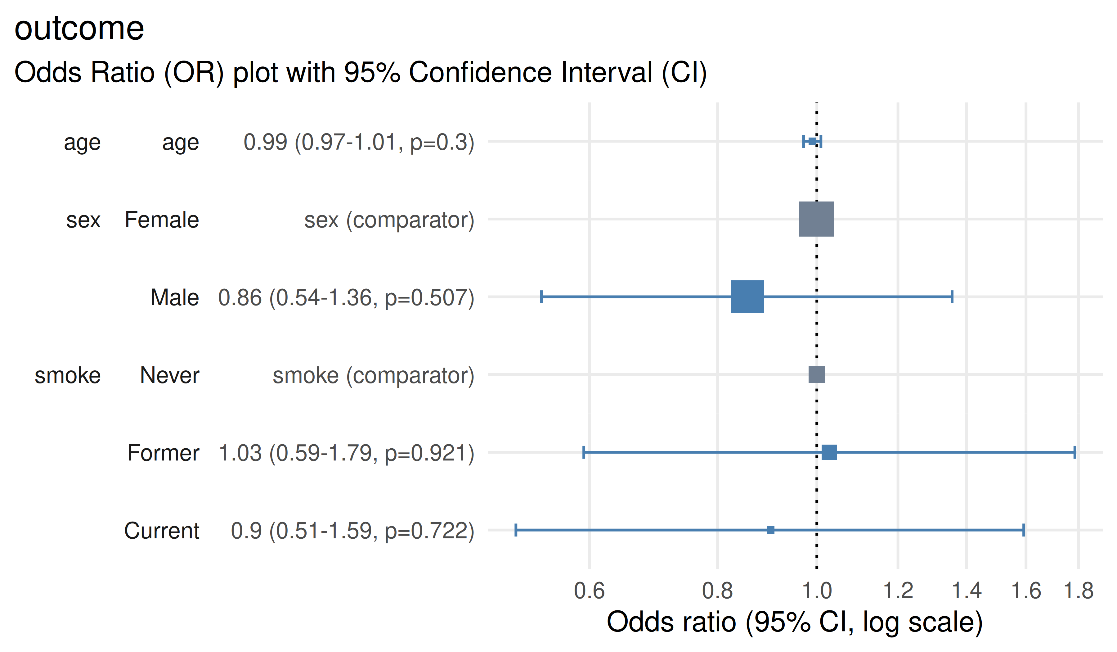
Quick interpretation
check_or()flags potential model issues. Concerns raised here should be a prompt for further investigative work to understand the implications for your model’s validity.table_or()provides odds ratios, 95% confidence intervals and p-values in a publication-friendly layout. Prefer reporting confidence intervals alongside point estimates rather than p-values alone.plot_or()visualises effect sizes and uncertainty. Interpret odds ratios > 1 as increased odds; odds ratios < 1 as decreased odds. If the confidence interval crosses 1, there is no clear evidence of an association at the chosen confidence interval level (default 95%).
See also
vignette("plot_or")- detailed plotting options and themesvignette("table_or")- formatting, gt integration and exportvignette("check_or")- diagnostics and case studies